CytoScan: automated flagging of technical anomalies for cytometry quality control
Tim R. Mocking
Amsterdam UMCFelix Zwolle
Amsterdam UMCYejin Park
Amsterdam UMCAngele Kelder
Amsterdam UMCYvan Saeys
VIB GhentJacqueline Cloos
Amsterdam UMCSofie van Gassen
VIB GhentCosta Bachas
Amsterdam UMCSource:
vignettes/CytoScan.Rmd
CytoScan.RmdAbstract
Studies evaluating cellular phenotypes by cytometry techniques are increasingly facing analytical challenges due to the multitudes of samples and parameters that are evaluated concurrently. However, spurious technical effects resulting from a lack of standardization can affect marker distributions and complicate multi-sample analyses. To identify such effects we present CytoScan, an R package that evaluates inter-measurement variation in cytometry datasets and allows for flagging anomalous measurements after data acquisition. CytoScan can detect two types of anomalies: files with limited similarity to others within a dataset (outliers) and files with limited similarity to previously acquired high-quality reference data (novelties). CytoScan can be applied to large cytometry datasets on consumer-grade hardware with informative visualizations, providing accessible quality-control for more reliable analyses.
Installation
CytoScan is currently only available from Github with the devtools package.
# Install devtools if needed
if (!requireNamespace("devtools", quietly = TRUE)) {
  install.packages("devtools")
}

devtools::install_github("AUMC-HEMA/CytoScan")## Warning: replacing previous import 'dplyr::count' by 'mclust::count' when
## loading 'CytoScan'Setting up a CytoScan workflow
The CytoScan package contains a function “generateDemo”. That generates a folder containing a small set of FCS files which will be used throughout this tutorial.
Loading demo data
# Create a folder "demo_data" containing 100 small FCS files for demonstration
# Each file contains 1000 events with 8 channels
generateDemo(dir = "demo_data", nFiles = 100, nCells = 1000, nChannels = 8)

# List the generated files
files <- list.files("demo_data", full.names = TRUE)
head(files, 3) # Show the names of the first 3 files
## [1] "demo_data/1.fcs" "demo_data/10.fcs" "demo_data/100.fcs"Initializing a CytoScan object
The first step in the workflow is creating a CytoScan object. This object stores all relevant information, from metadata, to file paths to generated features and outputs.
CS <- CytoScan()This “empty” object contains almost nothing at this point. It contains a function that defines the way will pre-process each FCS file and some variables to make this work with parallel processing. Modifying this is more advanced and will discussed later in this tutorial.
Let’s continue with adding some data.
Adding data to a CytoScan object
Adding FCS data
Every workflow depends on a set of “test” files. These are the files you want to evaluate for potential anomalies.
CS <- CytoScan() # Intialize empty object
files <- list.files("demo_data", full.names = TRUE) # Get file paths
CS <- addTestdata(CS, files) # Add file paths to object
If you want to perform novelty detection, you have to define reference data as well. In this case, models will be trained on the reference data, before identifying novelties in the test data.
CS <- CytoScan() # Intialize empty object
files <- list.files("demo_data", full.names = TRUE) # Get file paths
CS <- addReferencedata(CS, files[1:50]) # Add first 50 files as "test"
CS <- addTestdata(CS, files[51:100]) # Add last 50 files as "reference"
Adding metadata
You might also want to apply known experimental conditions such as the cytometer that was used or lot IDs. In the current version, we support adding one categorical label per file. You can add this to the object with the add label functions.
# Generate some random batches
refLabels <- sample(c("batch1", "batch2"), 50, replace = TRUE)
testLabels <- sample(c("batch1", "batch2"), 50, replace = TRUE)
head(refLabels)
## [1] "batch1" "batch2" "batch1" "batch2" "batch1" "batch1"
# Add them to the CytoScan object
CS <- addReferencelabels(CS, refLabels)
CS <- addTestlabels(CS, testLabels)
Inspecting the CytoScan object
Let’s inspect what the CytoScan object now looks like. We have different slots:
## [1] "preprocessFunction" "parallel"           "truncate_max_range"
## [4] "paths"              "labels"
You can see we know have added slots for “paths” and “labels” that we added with the add data and add label functions.
These paths are subdivided into test and reference categories:
## [1] "reference" "test"Inspecting these slots will reveal your input data. Note that we have not loaded any of the data yet. We just have made a structure for data loading that will be used later.
print((CS$paths$test))## [1] "demo_data/54.fcs" "demo_data/55.fcs" "demo_data/56.fcs" "demo_data/57.fcs"
## [5] "demo_data/58.fcs" "demo_data/59.fcs" "demo_data/6.fcs" "demo_data/60.fcs"
## [9] "demo_data/61.fcs" "demo_data/62.fcs" "demo_data/63.fcs" "demo_data/64.fcs"
## [13] "demo_data/65.fcs" "demo_data/66.fcs" "demo_data/67.fcs" "demo_data/68.fcs"
## [17] "demo_data/69.fcs" "demo_data/7.fcs" "demo_data/70.fcs" "demo_data/71.fcs"
## [21] "demo_data/72.fcs" "demo_data/73.fcs" "demo_data/74.fcs" "demo_data/75.fcs"
## [25] "demo_data/76.fcs" "demo_data/77.fcs" "demo_data/78.fcs" "demo_data/79.fcs"
## [29] "demo_data/8.fcs" "demo_data/80.fcs" "demo_data/81.fcs" "demo_data/82.fcs"
## [33] "demo_data/83.fcs" "demo_data/84.fcs" "demo_data/85.fcs" "demo_data/86.fcs"
## [37] "demo_data/87.fcs" "demo_data/88.fcs" "demo_data/89.fcs" "demo_data/9.fcs"
## [41] "demo_data/90.fcs" "demo_data/91.fcs" "demo_data/92.fcs" "demo_data/93.fcs"
## [45] "demo_data/94.fcs" "demo_data/95.fcs" "demo_data/96.fcs" "demo_data/97.fcs"
## [49] "demo_data/98.fcs" "demo_data/99.fcs"Feature generation
Before we can continue with visualizations and anomaly detection, we have to generate some features.
We recommend quantile-based features.
Note that you will have to supply the channel names in the function. If these do not match across files, the function will return an error.
General example
CS <- CytoScan()
files <- list.files("demo_data", full.names = TRUE)
CS <- addTestdata(CS, files)

channels <- LETTERS[1:8] # The channel names of demo_data are A-H
CS <- generateFeatures(CS, channels = channels, featMethod = "quantiles")
## Using 50% of cores: 2
head(CS$features$test$quantiles)## A_0.1 A_0.2 A_0.3 A_0.4 A_0.5
## demo_data/1.fcs -5.357358 -2.560892 0.1294535 0.9610448 1.6917434
## demo_data/10.fcs -6.954351 -5.684075 -4.6956966 -3.7656379 -2.5596028
## demo_data/100.fcs -4.871000 -1.203661 0.5407932 1.2339385 1.8912330
## demo_data/11.fcs -7.174882 -5.975318 -4.9984827 -4.1472255 -3.0097210
## demo_data/12.fcs -7.281292 -6.293276 -5.3656719 -4.7107177 -3.9825312
## demo_data/13.fcs -5.908609 -4.417424 -2.6406409 -0.1376041 0.9797448
## A_0.6 A_0.7 A_0.8 A_0.9 B_0.1 B_0.2
## demo_data/1.fcs 2.3633812 3.1734545 3.8303256 4.835522 -6.098922 -4.676040
## demo_data/10.fcs -0.6282217 1.3131984 2.6309642 3.955971 -7.348511 -6.065712
## demo_data/100.fcs 2.5208300 3.1463032 3.8631848 5.297232 -6.353052 -4.950840
## demo_data/11.fcs -1.7386829 0.4501492 1.9743166 3.554216 -4.703990 -1.581106
## demo_data/12.fcs -3.1039686 -1.9469767 0.1402388 2.714008 -6.953565 -5.659260
## demo_data/13.fcs 1.8884836 2.6809195 3.5772695 4.523193 -6.114951 -4.376585
## B_0.3 B_0.4 B_0.5 B_0.6 B_0.7
## demo_data/1.fcs -3.0698927 -0.2816961 0.8753238 1.716843 2.6432814
## demo_data/10.fcs -5.2320388 -4.4558579 -3.5108446 -2.402956 -0.7286981
## demo_data/100.fcs -3.8741315 -2.3388936 -0.1729573 1.231532 2.0497872
## demo_data/11.fcs 0.3373451 1.2063586 1.9302596 2.615487 3.2546176
## demo_data/12.fcs -4.6113813 -3.6304752 -2.3196097 -0.433030 1.1377957
## demo_data/13.fcs -2.9645786 -0.2173662 0.9321145 1.778016 2.6136120
## B_0.8 B_0.9 C_0.1 C_0.2 C_0.3 C_0.4
## demo_data/1.fcs 3.537842 4.715754 -6.432429 -5.243663 -4.111321 -2.8361613
## demo_data/10.fcs 1.382935 3.206491 -6.172819 -4.577787 -2.965015 -0.2639604
## demo_data/100.fcs 3.183651 4.429812 -6.262388 -4.806296 -3.444582 -1.5161178
## demo_data/11.fcs 3.967956 5.009612 -6.708834 -5.661523 -4.692090 -3.7262715
## demo_data/12.fcs 2.557733 3.952181 -7.214981 -6.236087 -5.546532 -4.7146389
## demo_data/13.fcs 3.514837 4.848460 -7.425417 -6.332052 -5.491508 -4.7928229
## C_0.5 C_0.6 C_0.7 C_0.8 C_0.9 D_0.1
## demo_data/1.fcs -1.0251901 0.92667064 1.925871 2.9319616 4.302333 -6.504877
## demo_data/10.fcs 0.9854750 1.86285518 2.726433 3.5284368 4.568450 -6.426312
## demo_data/100.fcs 0.3581515 1.34057582 2.239483 3.2516853 4.238098 -5.651842
## demo_data/11.fcs -2.3853820 -0.03843239 1.501512 2.7221638 4.032346 -6.835155
## demo_data/12.fcs -3.9595126 -3.02865284 -1.985451 0.6203027 2.788029 -6.597431
## demo_data/13.fcs -4.1030718 -3.15960509 -2.123862 0.4823559 2.522719 -6.857977
## D_0.2 D_0.3 D_0.4 D_0.5 D_0.6
## demo_data/1.fcs -5.308050 -4.1428152 -3.0521902 -0.94694714 0.6932152
## demo_data/10.fcs -4.904924 -3.3769336 -0.9195361 0.82631950 1.7876462
## demo_data/100.fcs -3.331257 -0.8326616 0.5943932 1.44264178 2.1554972
## demo_data/11.fcs -5.543317 -4.4699051 -3.3009377 -1.40786696 0.5983005
## demo_data/12.fcs -5.262169 -3.9481912 -2.3776900 0.08347005 1.2848876
## demo_data/13.fcs -5.743191 -4.8999460 -4.0104448 -3.09688910 -1.5534788
## D_0.7 D_0.8 D_0.9 E_0.1 E_0.2 E_0.3
## demo_data/1.fcs 1.8025224 2.841113 4.412030 -5.223580 -2.476540 0.3001880
## demo_data/10.fcs 2.5824877 3.446907 4.866182 -7.095521 -5.883702 -5.0838944
## demo_data/100.fcs 3.0030478 3.840990 4.959328 -7.258486 -6.127407 -5.3075216
## demo_data/11.fcs 1.8330571 3.085947 4.306980 -5.340485 -3.242215 -0.8132622
## demo_data/12.fcs 2.2480667 3.164973 4.332617 -7.138573 -5.943941 -5.2876535
## demo_data/13.fcs 0.7240487 2.293197 3.808449 -6.378070 -5.037289 -3.9352150
## E_0.4 E_0.5 E_0.6 E_0.7 E_0.8 E_0.9
## demo_data/1.fcs 1.1191788 1.7425821 2.412758 3.0168422 3.8061640 4.832398
## demo_data/10.fcs -4.0229573 -3.0806520 -1.728079 0.3797487 2.0714221 3.884998
## demo_data/100.fcs -4.6549513 -3.8694639 -3.137098 -2.1138309 0.0158442 2.747227
## demo_data/11.fcs 0.6843694 1.3603094 2.252671 2.9443782 3.8015649 4.854079
## demo_data/12.fcs -4.3990474 -3.3787366 -2.581126 -0.9604667 1.2795781 3.087591
## demo_data/13.fcs -2.1343228 0.2645146 1.484844 2.2265876 3.1855266 4.481376
## F_0.1 F_0.2 F_0.3 F_0.4 F_0.5 F_0.6
## demo_data/1.fcs -7.138807 -6.018600 -5.0491165 -4.1883346 -3.377373 -2.405154
## demo_data/10.fcs -4.868278 -2.220064 0.2103583 1.1334219 1.800293 2.424347
## demo_data/100.fcs -5.888807 -3.969304 -1.0938682 0.4703571 1.323663 2.105145
## demo_data/11.fcs -6.948860 -5.875529 -5.0111194 -4.1324493 -3.417655 -2.280095
## demo_data/12.fcs -7.282769 -6.000755 -5.0739703 -4.0418013 -3.127304 -1.911529
## demo_data/13.fcs -6.699588 -5.244856 -4.2597360 -3.0559867 -1.229603 0.844851
## F_0.7 F_0.8 F_0.9 G_0.1 G_0.2 G_0.3
## demo_data/1.fcs -0.3136551 1.660059 3.421149 -5.397980 -3.483239 -0.9541440
## demo_data/10.fcs 3.1537132 3.904394 5.004978 -6.489649 -5.322838 -3.9982362
## demo_data/100.fcs 2.8559552 3.793556 4.953506 -7.073208 -6.051633 -5.0991057
## demo_data/11.fcs -0.5372557 1.718757 3.232754 -5.479251 -3.329701 -0.4247143
## demo_data/12.fcs 0.4568697 2.113952 3.668121 -6.362546 -4.448574 -2.8001686
## demo_data/13.fcs 1.8893505 2.998695 4.393250 -7.056078 -6.109151 -5.2248003
## G_0.4 G_0.5 G_0.6 G_0.7 G_0.8 G_0.9
## demo_data/1.fcs 0.4975959 1.2996444 1.992819 2.7992631 3.727629 4.785652
## demo_data/10.fcs -2.8603597 -0.4061297 0.989262 1.8729830 2.897811 4.387560
## demo_data/100.fcs -4.3410818 -3.2306743 -1.961519 0.2116263 1.810068 3.474658
## demo_data/11.fcs 0.8296125 1.4766762 2.216793 2.9074561 3.746310 4.942874
## demo_data/12.fcs 0.1141107 1.1292142 1.807748 2.4941949 3.280671 4.470439
## demo_data/13.fcs -4.5575167 -3.5869585 -2.557901 -0.7286524 1.562600 3.468623
## H_0.1 H_0.2 H_0.3 H_0.4 H_0.5
## demo_data/1.fcs -6.215254 -4.565840 -2.5769806 -0.07129956 0.8895623
## demo_data/10.fcs -6.815182 -5.949652 -5.1019786 -4.40642099 -3.4696945
## demo_data/100.fcs -6.037355 -4.259865 -2.2202496 0.02789772 0.9374362
## demo_data/11.fcs -7.331584 -6.003219 -5.2201818 -4.38422432 -3.5724715
## demo_data/12.fcs -5.461581 -3.305407 -0.3669578 0.68057348 1.4535415
## demo_data/13.fcs -4.940050 -2.579636 0.2850174 1.08213267 1.6309281
## H_0.6 H_0.7 H_0.8 H_0.9
## demo_data/1.fcs 1.628342 2.5475950 3.542617 4.806489
## demo_data/10.fcs -2.367702 -0.2619296 1.644831 3.289412
## demo_data/100.fcs 1.727217 2.6418914 3.361925 4.599191
## demo_data/11.fcs -2.545524 -0.7707796 1.652821 3.516051
## demo_data/12.fcs 2.090857 3.0188223 3.812906 5.010687
## demo_data/13.fcs 2.349348 3.0102229 3.855929 4.927961Note that by default, the function will use 50% of your cores for parallel processing. However, this is only really necessary for larger datasets. You can disable parallel processing with the “parallel” argument. You can also define the number of cores with “cores”.
If you run generateFeatures again, CytoScan will not do anything. This is because it automatically detects if all the files have generated features. If you want to run the function again, you can force it with “recalculate”.
# This will not do anything... (assuming you already generated quantile features)
CS <- generateFeatures(CS, channels = channels, featMethod = "quantiles")

# Force CytoScan to recalculate features for previous supplied files
CS <- generateFeatures(CS, channels = channels, featMethod = "quantiles",
                       recalculate=TRUE)
This also means that you can add additional test and reference files and generate features just for these new files. This makes the workflow a lot more flexible.
CS <- CytoScan()
CS <- addTestdata(CS, files[0:50])
channels <- LETTERS[1:8]

# Generate features for the first 50 files
CS <- generateFeatures(CS, channels = channels, featMethod = "quantiles")
print(nrow(CS$features$test$quantiles))

# Now add the other 50 files
CS <- addTestdata(CS, files[51:100])
CS <- generateFeatures(CS, channels = channels, featMethod = "quantiles")
print(nrow(CS$features$test$quantiles))
Generating features for novelty detection
If you want to perform novelty detection, you have to generate features from the reference cohort. In this example, we use the earth mover’s distance (EMD) for feature generation. Because these distances are calculated based on an aggregated set of cells, it is important to use cells from the reference cohort.
If reference data is present, this is automatically used for aggregation.
CS <- CytoScan()
CS <- addTestdata(CS, files[1:50])
CS <- addReferencedata(CS, files[51:100])
CS <- generateFeatures(CS, channels = channels, featMethod = "EMD")
Visualizations
Let’s make some visualizations.
# General set-up with some test and reference data
CS <- CytoScan()
CS <- addTestdata(CS, files[1:50])
CS <- addReferencedata(CS, files[51:100])
CS <- generateFeatures(CS, channels = channels, featMethod = "quantiles")
## Using 50% of cores: 2Principal component analysis (PCA)
Plotting the principal components is one of the easiest ways to visualize the patterns in your dataset. The “plotPCA” function is quite versatile. It has three mandatory arguments:
- featMethod
- fitData
- plotData
featMethod defines which features to plot. This is to deal with situations where you generated features for both quantiles and EMD.
fitData defines which data source to use for calculating the PCs. This allows you to “project” data from test samples in a reference set PCA, etc.
plotData defines which data to plot. This allows you to plot only test or reference, or all samples.
# Plot a PCA for only the test samples
plotPCA(CS, featMethod = "quantiles", fitData = "test", plotData = "test")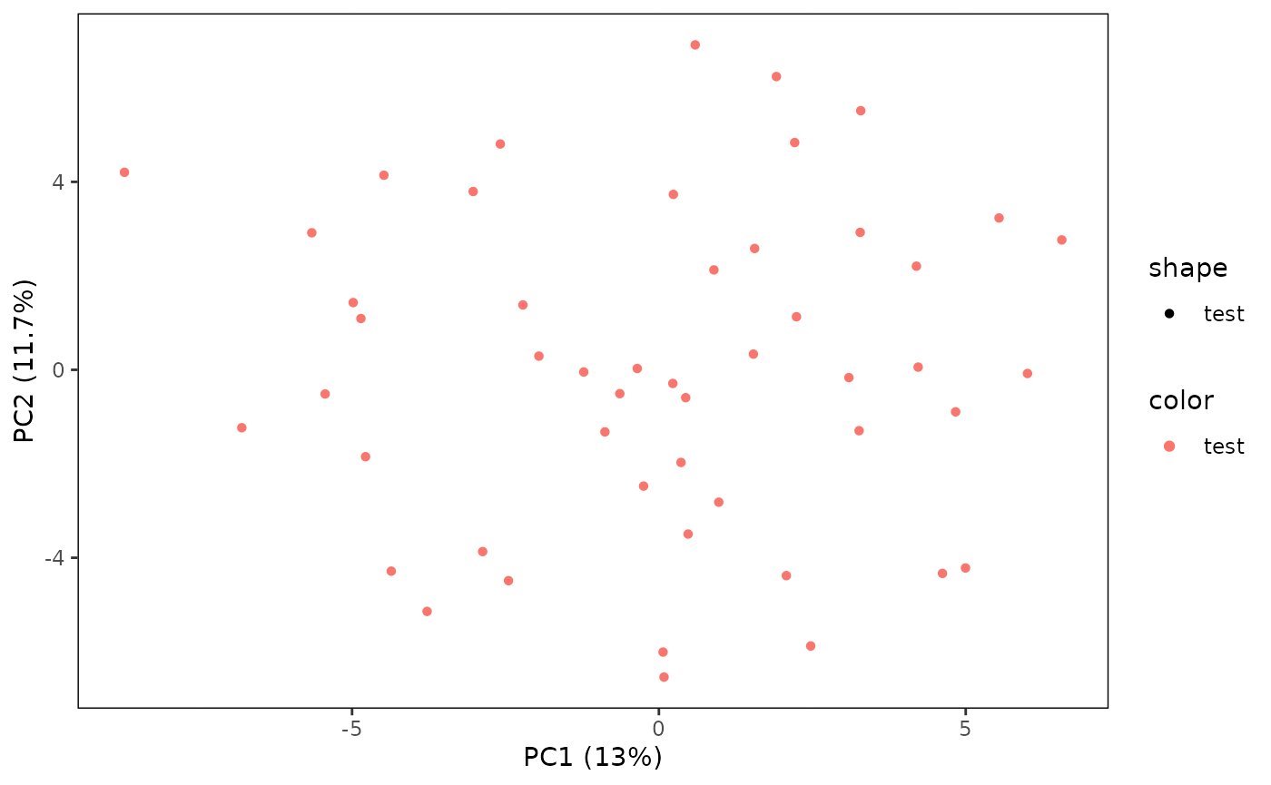
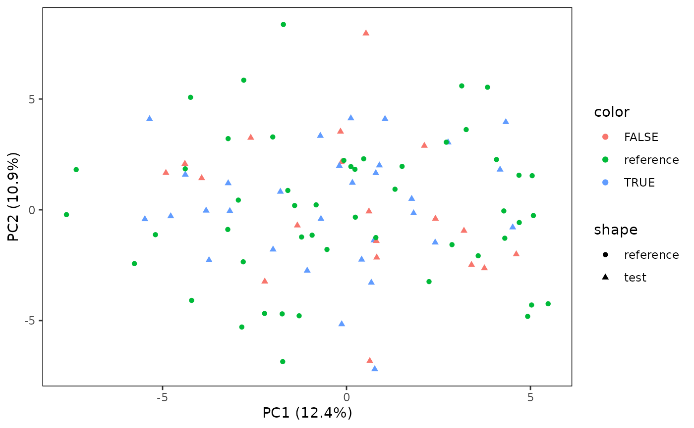
# Also plot the reference samples
plotPCA(CS, featMethod = "quantiles", fitData = "test", plotData = "all")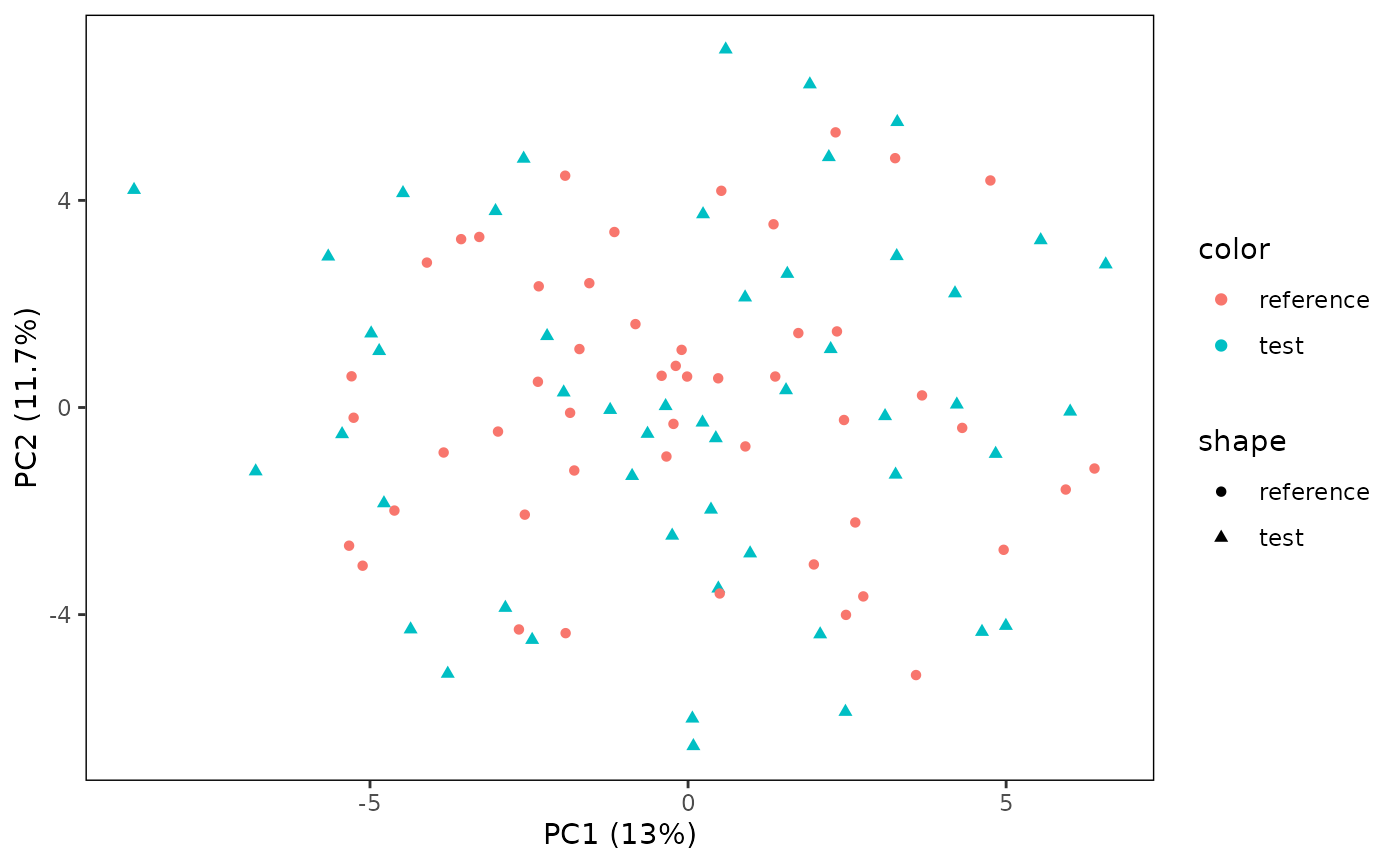
You can also define the PCs you want to plot on the x and y-axes. Here, we change it to PC3 and 4.
# Plot PC3 vs. PC4
plotPCA(CS, featMethod = "quantiles", fitData = "test", plotData = "all", PCx = 3, PCy = 4)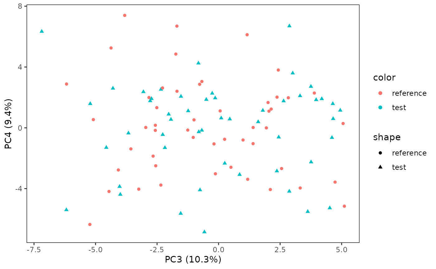
Sometimes, you are interested in which features influence the orientation of the PCA plot. You can evaluate this with two ways.
The first method is to plot the loadings within the plot. This can be set-up with “plotArrows”. However, as we have many features, it sometimes makes sense to only plot the first couple of important ones (“nLoadings”).
# Plot the direction of the most influential feature
plotPCA(CS, featMethod = "quantiles", fitData = "test", plotData = "all",
        plotArrows = TRUE, nLoadings = 1)
## Warning: Using `size` aesthetic for lines was deprecated in ggplot2 3.4.0.
## ℹ Please use `linewidth` instead.
## ℹ The deprecated feature was likely used in the CytoScan package.
## Please report the issue at <https://github.com/AUMC-HEMA/CytoScan/issues>.
## This warning is displayed once per session.
## Call `lifecycle::last_lifecycle_warnings()` to see where this warning was
## generated.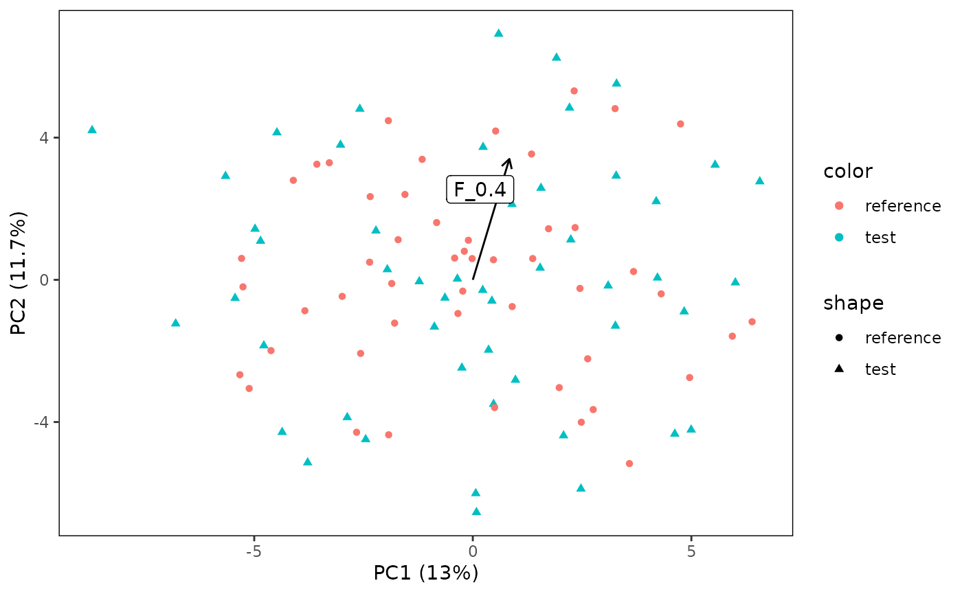 You can also create a barplot alongside the x and y-axis to show which
features influence the PCs plotted on the x and y axis.
You can also create a barplot alongside the x and y-axis to show which
features influence the PCs plotted on the x and y axis.
plotPCA(CS, featMethod = "quantiles", fitData = "test", plotData = "all",
        plotBars = TRUE, nLoadings = 10)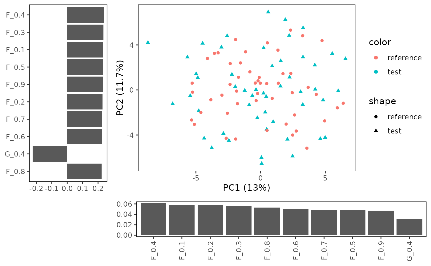
## TableGrob (2 x 2) "arrange": 4 grobs
##   z     cells    name           grob
## 1 1 (1-1,1-1) arrange gtable[layout]
## 2 2 (1-1,2-2) arrange gtable[layout]
## 3 3 (2-2,1-1) arrange gtable[layout]
## 4 4 (2-2,2-2) arrange gtable[layout]
Lastly, we can control the shape and color used by the plot. We will add some experimental conditions and color those, while retaining the distinction between test and reference by shape.
refLabels <- sample(c("batch1", "batch2"), 50, replace = TRUE)
testLabels <- sample(c("batch1", "batch2"), 50, replace = TRUE)
CS <- addReferencelabels(CS, refLabels)
CS <- addTestlabels(CS, testLabels)
plotPCA(CS, featMethod = "quantiles", fitData = "test", plotData = "all",
        color = "labels")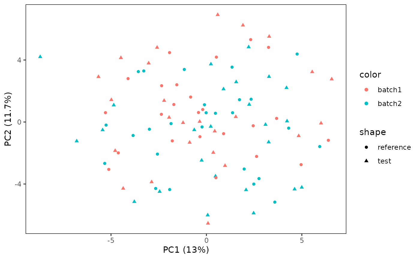
Advanced customization of PCA plots
The lay-out and colors of the plot might not be “publication ready”. However, because the plot function returns a ggplot object, you can modify according to your own desire.
p <- plotPCA(CS, featMethod = "quantiles", fitData = "test", plotData = "all",
             color = "labels")

# Modify ggplot settings
library(ggplot2)
p <- p +
  scale_color_manual(values = c("batch1" = "red", "batch2" = "blue"))
plot(p)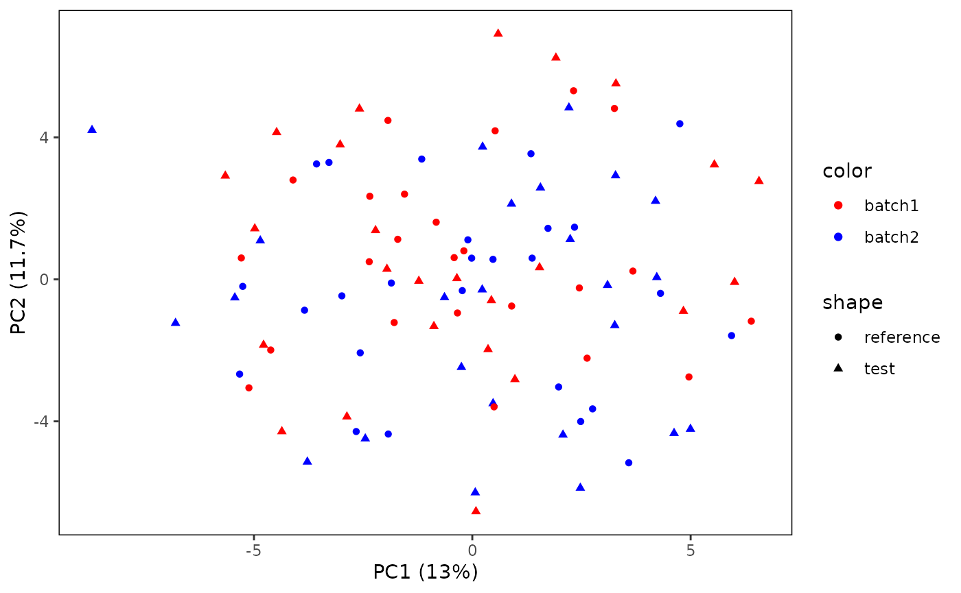
Heatmaps
You can also plot the featurers in a heatmap. We use the ComplexHeatmap package.
plotHeatmap(CS, featMethod = "quantiles", plotData = "test")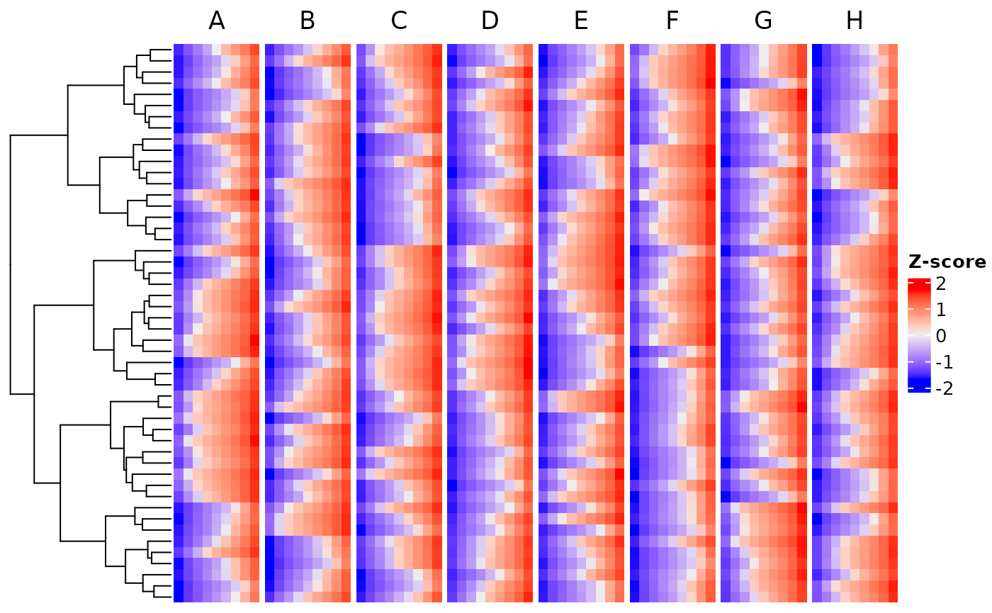
Boxplots
You can also plot specific channel distributions.
Here, we plot the expression of the hypothetical marker “A”. You can see, that for plotting all files, the plot becomes crowded very fast.
plotBoxplot(CS, plotData = "all", channel = "A")##
## Attaching package: 'dplyr'## The following object is masked from 'package:flowCore':
##
## filter## The following objects are masked from 'package:stats':
##
## filter, lag## The following objects are masked from 'package:base':
##
## intersect, setdiff, setequal, union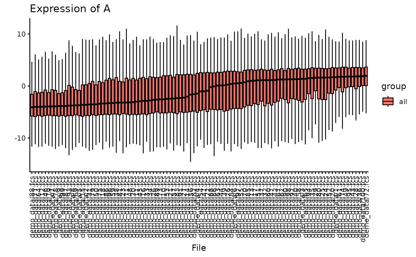 Therefore, you can also decide to plot only random subset of the files
for larger datasets.
Therefore, you can also decide to plot only random subset of the files
for larger datasets.
plotBoxplot(CS, plotData = "all", channel = "A", nFiles = 30)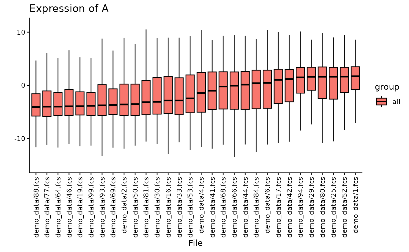
You can also highlight the source of the data. As you can see here, the files are sorted from median low to high, and the two subsets are quite well mixed.
plotBoxplot(CS, plotData = "all", channel = "A", nFiles = 30, color = "input")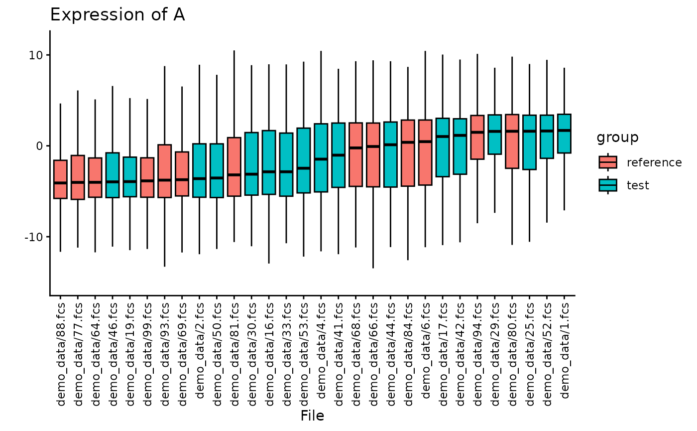
Flagging anomalies
Now let’s figure out if we have any anomalies. For this, we use the “Flag” function.
You always need to define based on which feature set you want to flag anomalies.
Flagging anomalies using outlier detection
CS <- CytoScan()
CS <- addTestdata(CS, files[0:50])
CS <- addReferencedata(CS, files[51:100])
CS <- generateFeatures(CS, channels = channels, featMethod = "quantiles")
## Using 50% of cores: 2
# Flag outliers
# Note: we slightly modified the cut-off due to the unrealistic simulated setting
CS <- Flag(CS, featMethod = "quantiles", flagMethod = "outlier",
           outlier_threshold = 0.52)
You can identify the outliers in the CytoScan object.
head(CS$outliers$quantiles)## demo_data/1.fcs demo_data/10.fcs demo_data/100.fcs demo_data/11.fcs
## FALSE FALSE FALSE FALSE
## demo_data/12.fcs demo_data/13.fcs
## FALSE FALSE
## Levels: FALSE TRUEFlagging anomalies using novelty detection
CS <- Flag(CS, featMethod = "quantiles", flagMethod = "novelty")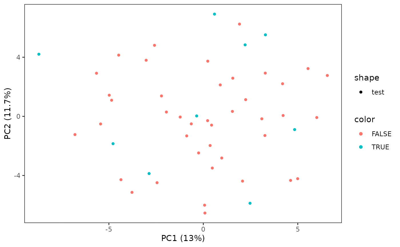
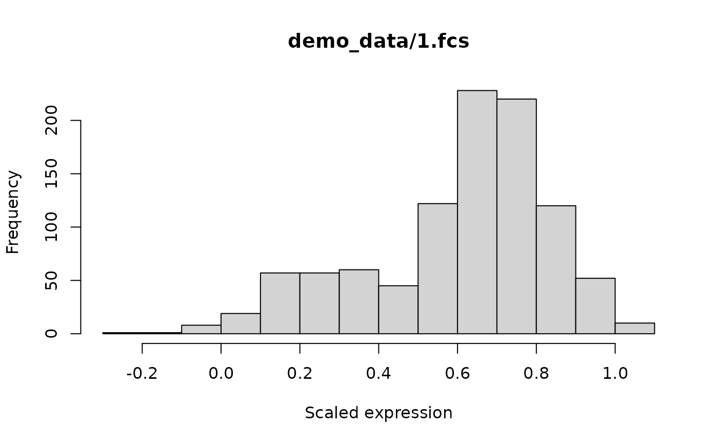
Custom pre-processing
By default, CytoScan uses the same pre-processing function for all loaded flowframes.
You can modify this by supplying your own pre-processing function, for example by only performing a MinMax normalization.
CS <- CytoScan()

# Define a custom function which also scales expression values from 0 to 1
MinMax <- function(ff){
  spill <- ff@description$SPILL
  ff <- flowCore::compensate(ff, spill)
  ff <- flowCore::transform(ff, flowCore::transformList(colnames(spill),
                                            flowCore::arcsinhTransform(a = 0,
                                                                       b = 1/150,
                                                                       c = 0)))
  ff@exprs[, colnames(spill)] <- apply(ff@exprs[, colnames(spill)], 2, function(x){
    return((x - quantile(x, 0.01)) / (quantile(x, 0.99) - quantile(x, 0.01)))
  })
  return(ff)
}

# Replace the default pre-processing
CS$preprocessFunction <- MinMax

# Read some data
CS <- addTestdata(CS, files[1], read = TRUE, aggSize = 1000)

# Plot a histogram of the first marker
hist(CS$data$test[[files[1]]][, 1], main = files[1], xlab = "Scaled expression")